Algorithm for the experience

Set the initial values N=30000, I=10. We make the conservative choice of . For every define n(i)=100i and .

1. Assign d=1.
2. Assign i=1.
3. Assign m=1.
4. Assign a(m)=(m-1)n(i).
5. Generate , sampling from the random vector with cummulative distribution function if d=1, and with if d=2.
6. Assign and calculate
   • ,
   • ,
   • ,
   • and
   • .
7. If m=M(i) continue in step E8. Else, assign m=m+1 and return to step E4.
8. If i=I continue in step E9. Else, assign i=i+1 and continue in step E3.
9. If d=2 continue in step E10. Else, assign d=d+1 and continue in step E2.
10. For every d=1,2 and every define the following vectors:
    • ,
    • ,
    • ,
    • and
    • .
    Analyze the empirical distributions of every vector defined above.
11. Show the results in a table, for example following the presentation suggested in Lewis and Orav (1989), clearly stating:
    • Distribution generated.
    • Total size of the sample observed from the distribution, for every , say N.
    • Sample size upon which the pocedures are based: .
    • Number of observed procedures for every value of , say . Note that

       

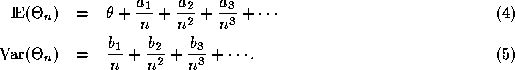
Formula (3) is required because under certain hypothesis (see, for example, Lehmann (1983)), the following asymptotic expansions hold:

  

If that is the case, one could carry on analyzing the regression model defined by:

 

where estimator of , ``sample mean'' over samples of of size M(i), , , , . Here, represents any of the (100 in total).

Now, since we have from equation (5) that, for n(i) large:

using equation (4). Thus, . Moreover, taking into account the simulation scheme, we might consider that are independent (notice that, for each the generation proceeds, instead of going back to the beginning).

We can then apply a regression analysis to the model (6) considering the values as the observed values of . Then, for example using least squares estimators, we could estimate the coefficients in (6) with

 

In order to assess the accuracy of the estimators in (7), the simulation could be carried on obtaining, say R, values like

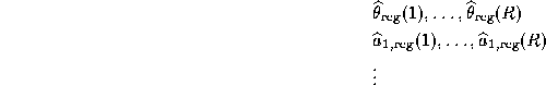
Then, one could analyze the empirical distributions of

and, from this, we would obtain estimates of the accuracy of the least squares estimators in model (6). Remember that, in most of the situations, our main goal will be knowledge about ; but is also interesting since it says something about the asymptotic bias of the procedure.

Observe that, after performing those R replications we will have at hand RM(i) outcomes of the random variable : . This sample would allow us to study its empirical distribution. We omit this last part in this work.