
Demonstration by Pedro M. M. de Castro.
We would like to thank Jane Tournois, Pierre Alliez and Olivier Devillers. Tools for computational exploration and implementation: OpenAI Codex and Anthropic Claude.
Moving a vertex without changing its connections
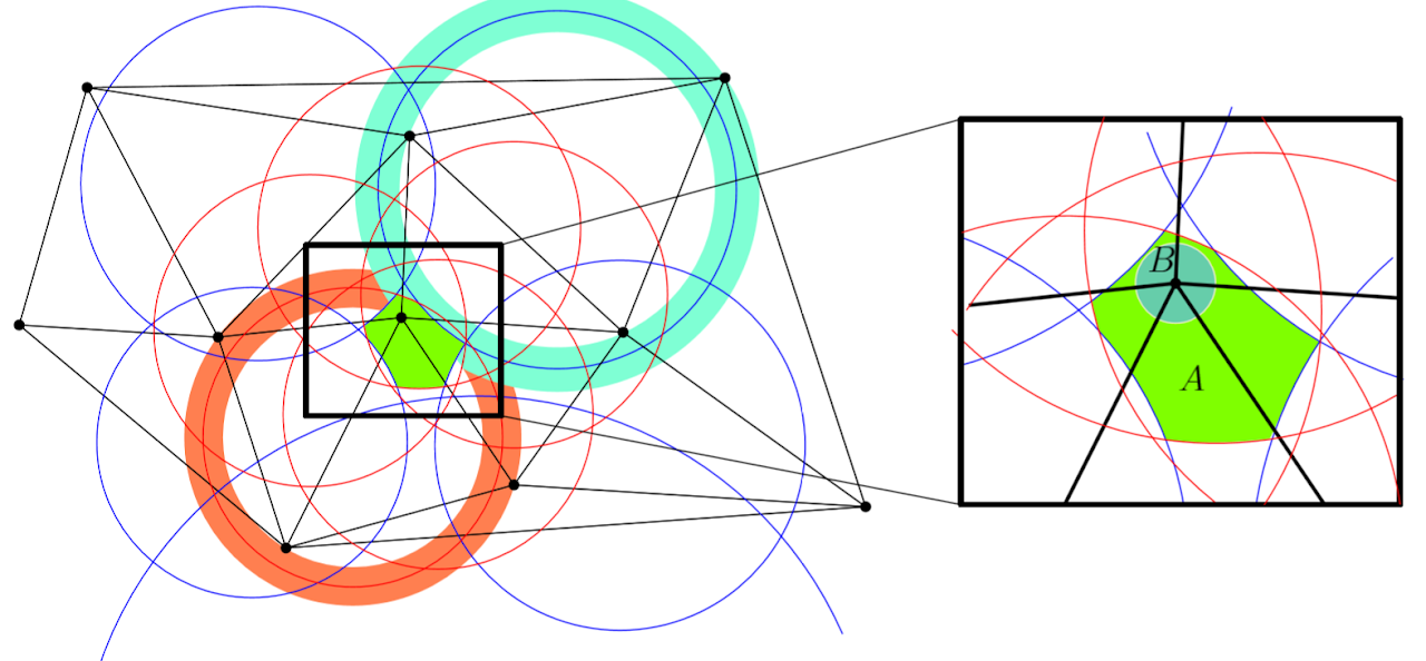
Derived from Filtering Relocations on a Delaunay Triangulation, by Pedro Machado Manhães de Castro, Jane Tournois, Pierre Alliez and Olivier Devillers, Computer Graphics Forum 28(5), 1465–1474 (2009). The complete region A and the centered disk B correspond to Figure 3 and §§2.2–2.3.
Read the paper · Public full text · Illustrated research account
Application: bounded centroidal Voronoi tessellation
Section 4.1, “Clustering”, pp. 1470–1471, Equation (5) and Figures 5–7 describe Lloyd iterations: integrate a Voronoi partition to obtain its centroids, relocate the sites to those centroids, then recompute the partition. Figure 5 uses 1,000 points in a disc and 1,000 iterations. The present walkthrough uses the chosen point set, a fixed enclosing rectangle Ω and uniform density ρ = 1. These are explicit teaching choices, not a reproduction of the paper’s experiment.
For each site pᵢ, its cell is Ω intersected with all half-planes |x − pᵢ|² ≤ |x − pⱼ|². Polygon area and first moments give its centroid. For the walkthrough, polygon second moments give the site-based energy E(P) = Σᵢ ∫Vᵢ |x − pᵢ|² dx. When sites coincide with their cell centroids, this agrees with the centroid form of Equation (5). The displayed energy is E / (area(Ω) D²), where D is the domain diagonal. Clipping, moments and display use a common isotropic normalization; no raster sampling or independent axis stretching is used. Each distinct position supplies one site; observation multiplicities are not density weights.
All centroid targets are computed from the same partition and frozen for the iteration. Together is the default: all sites are animated toward these frozen targets, with the Delaunay triangulation, bounded Voronoi cells and tolerance regions recomputed at each displayed intermediate configuration. One by one exposes the individual relocations. Neither mode recomputes target centroids between relocations. Both produce the same standard Lloyd update at the end of a full iteration. Its energy cannot increase in exact arithmetic; no monotonicity claim is made for the intermediate partially relocated configurations.
In One by one, each displayed disk test uses the configuration immediately before that single relocation; the dashed disk is that previous B and solid regions belong to the current configuration. In Together, the B count comes from a separate sequential replay of the remaining frozen-target relocations, refreshing the reference before each single move. It does not test or certify the simultaneous interpolation. Its intermediate disks are not overlaid on the simultaneous view. The count is exposed only when the atomic batch completes; displayed intermediate cells and regions all belong to the interpolated positions. Energy and residual remain those of the last completed iteration. The demo rebuilds and validates every resulting Delaunay triangulation. It illustrates eligibility for filtering; it does not implement the paper’s persistent fixed/moving references and repair queue, nor measure acceleration. A collection of individual tests against different references is not presented as a simultaneous common-reference guarantee. Outside B does not imply a change of connectivity.
The stopping test is maxᵢ |pᵢ − centroid(Vᵢ)| / D ≤ 10⁻⁴ after a completed iteration, with a limit of 200 iterations. This reports numerical stationarity at the chosen scale, not certified convergence or a global optimum. Cells must resolve to positive area; coincident numerical targets and inconsistencies stop the step. Energy checks use a scale-aware heuristic floating-point allowance. The pre-existing binary64 construction and heuristic filter limitations still apply. The rectangular boundary clips the Voronoi integration domain; it does not redefine the complete tolerance regions.
A: the intersection of permitted sides
A bi-cell consists of two adjacent triangles. Their shared-edge endpoints lie on one circle and the opposite vertices on another concentric circle. The standard delimiter is the circle halfway between these two radii. Each shared-edge endpoint must remain inside it; each opposite vertex must remain outside it.
Adjacent triangles: abc and abd, shared edge ab.
2 (d-c) · o = |d|² - |c|²
The region of a vertex is the intersection of the permitted sides of every bi-cell containing it, including bi-cells in which it is an opposite vertex. Near the convex hull, infinite bi-cells introduce straight median delimiters. The viewport never defines a boundary of the region.
This construction supports simultaneous movements within the reference regions. It is not the maximal region available to a single moving vertex when all other points are held fixed. Moving outside A can preserve or change the triangulation.
B: the largest disk centered at z₀
The center is fixed at the reference vertex. The radius is the smallest distance from that center to a delimiter. This gives the largest disk at that center contained in A. It does not search for a larger circle with a different center.
Closed boundaries are drawn, but positions on a boundary or within an uncertainty band receive no strict preservation guarantee. In Fixed reference mode, regions stay at the adopted positions. Selecting a vertex does not change that reference. Adopt current Delaunay installs the current triangulation as a new reference. Undo and Redo restore both points and their corresponding reference.
Fixed and live regions
Fixed reference compares positions with regions of the last explicitly adopted triangulation. The preservation condition concerns all vertices in their respective fixed regions. Live regions recomputes the triangulation and displayed regions together for each sampled movement frame. A point at the center of its freshly recomputed region does not certify that its movement preserved connectivity. Live mode makes no preservation claim; connectivity is compared separately with the adopted triangulation. Intermediate changes between sampled frames are not enumerated.
Reading the diagrams
Solid gray lines show Delaunay edges; dashed neutral lines show Voronoi edges. Green marks A and turquoise marks B. When Delimiters is enabled, red circles mean “stay inside,” blue circles mean “stay outside,” and ochre lines mark half-plane constraints. Both infinite bi-cell types from the article are included. Show all regions adds the other vertices’ region outlines while the selected region stays filled. A and B can be hidden independently. Unbounded or unavailable regions are identified explicitly.
A hull region may be unbounded. Its view is explicitly labeled partial. Fit frames a bounded region, while zooming only changes the camera. Mouse background dragging pans. On a touchscreen, tap a vertex to select it, then drag the selected vertex to move it. Swipe elsewhere to scroll the page and use two fingers to zoom and pan without moving points.
Finite precision and exceptional inputs
Delaunay connectivity is reconstructed independently after each accepted move, using filtered predicates with an exact integer fallback on the represented binary64 coordinates. Circles, intersections and region membership use finite-precision numerical constructions. The uncertainty estimate is heuristic and is not a certified error bound, especially when a point set contains very different scales.
Large or ill-conditioned constructions may be suppressed with a visible “no guarantee” message. If numerical membership and rebuilt connectivity disagree, the region is hidden and the disagreement is reported. The implementation does not use the displayed disk to skip triangulation updates.
Collinear sets have no two-dimensional region. Cocircular points can admit multiple Delaunay diagonals. Coincident input points are grouped with a notice, and a movement onto another point is rejected. The input limit is 150 points. See the complete specification and numerical conventions for the formulas, thresholds and limitations.
Measured examples
The preset menu includes Palmer penguin bills from 2007 (mm), Iris sepals from the corrected UCI dataset (cm), and NOAA water-level station locations in Florida and Texas (km after a local spherical azimuthal equidistant projection). The geographic examples are planar approximations, not geodesic Delaunay triangulations. Coincident pairs retain their observation counts; no jitter or unequal axis scaling is applied. Measured values at a fixed decimal resolution often contain exactly cocircular quadruples; the affected regions then have no guaranteed interior and the triangulation is reported as non-unique. Each preset exposes source, license, units, subset and transformation. Moved coordinates are marked as edited positions for exploration.
Sources and credits
The earlier paper Fast Delaunay Triangulation for Converging Point Relocation Sequences, by Castro and Devillers (EuroCG 2009, pp. 231–234), is a precursor. Chapter 5 of Castro's 2010 thesis, Practical Ways to Accelerate Delaunay Triangulations, gives a corresponding account. The full four-author CGF article is the principal source for this demonstration.
Typography uses Inter and Latin Modern, with the same local font files as the academic site and its point-location demonstration. Inter license · Latin Modern license. The CIn identity and academic navigation follow the academic site.